AI Engineer Interview Masterclass

The AI Engineer Interview Masterclass

The Definitive Technical Roadmap, Deep Dives, Interviewer Q&A Cards & System Design Playbook • Version 3.0

The Staff Engineer Philosophy
Part I: Foundations (The First-Principles Baseline)
Part II: Core Mechanics (The Intermediate Engine)
Part III: Production & Advanced AI (Scale & Serving)
Part IV: Frontier Scaled Architectures (Elite Self-Study)
Part V: The AI System Design Playbook & Worked Case Studies
Part VI: Interview Questions & Answers

The Staff Engineer Philosophy

Junior and mid-level candidates recite buzzwords and memorize API calls. Staff and Principal engineers evaluate trade-offs from first principles under real-world production constraints. In every technical and system design round, your objective is to explain:

What problem does each component solve? (Never draw a component without explaining what failure mode it eliminates).
How does it function internally? (Articulate the memory-bandwidth, cache hierarchy, and tensor dynamics).
Why were competing alternatives rejected? (Compare against baselines across latency, cost, and complexity).
What failure modes emerge at scale? (Diagnose silent degradation, drift, and security vectors).
How will you quantitatively measure production health? (Define exact offline benchmarks and online telemetry).

AI engineering lifecycle: define, build, evaluate, deploy, and monitor

Part I: Foundations (The First-Principles Baseline)

1.1 ML vs. Deep Learning vs. Generative AI

Artificial Intelligence spans three nested layers of capability:

Artificial Intelligence (AI): Any technique enabling machines to mimic intelligent behavior (symbolic logic, heuristic search, planning, expert systems).
Machine Learning (ML): Systems that discover statistical patterns from empirical data without hand-coded rules (Linear Regression, Random Forests, XGBoost).
Deep Learning (DL): ML leveraging multi-layered artificial neural networks that automatically extract hierarchical representations directly from raw unstructured inputs (CNNs, LSTMs, Transformers).
Generative AI (GenAI): Deep Learning models that model high-dimensional data distributions to generate novel text, audio, images, or code (GPT-4, Claude 3.5, Llama 3, Midjourney).

The Mathematical Distinction: Discriminative vs. Generative

Discriminative Models: Learn the conditional probability distribution **P(y

x)**. They optimize decision hyperplanes to partition existing data into discrete classes or continuous scalars (e.g., Logistic Regression, ResNet, BERT).

Generative Models: Capture the joint probability distribution P(x, y) or the high-dimensional autoregressive conditional token distribution: $P(\text{next\_token} \mid \text{context}) = \text{Softmax}\left(\frac{z_i}{\tau}\right)$ By modeling the underlying data-generating surface, they can sample entirely new, synthetic data points that follow the statistical regularities of the training corpus.

Tabular vs. Unstructured Decision Matrix

INTERVIEW PROMPT: “How do you determine whether a business problem requires Classical ML, Deep Learning, or Generative AI?”

CANDIDATE SOUNDBITE (60s): “I evaluate along three vectors: data modality, latency budget, and explainability constraints. For structured tabular records (e.g., fraud scoring, churn prediction), I deploy Gradient Boosted Trees (XGBoost/LightGBM) because they converge faster, provide deterministic latency, and allow exact feature importance audits. For raw unstructured inputs like computer vision or speech, I employ Deep Learning architectures to bypass manual feature extraction. I only introduce Generative AI when the problem strictly requires creative content synthesis, open-domain semantic understanding, or dynamic code generation.”

RED FLAG TRAP TO AVOID: Recommending an LLM for structured tabular credit risk or pricing problems. It demonstrates a lack of cost-awareness and architectural maturity.

1.2 The Production AI Project Lifecycle & Drift Dynamics

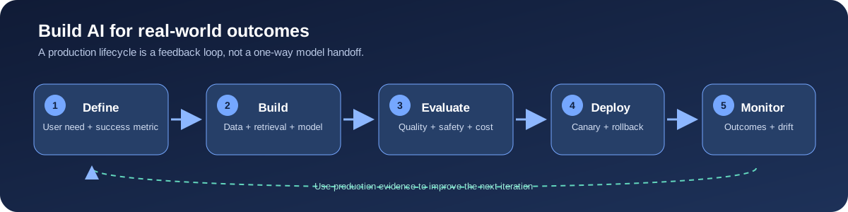
In production, model prototyping is 10% of the effort; 90% is building data pipelines, drift detection systems, evaluation gates, and serving infrastructure.

The 7 Production Stages:

Problem Definition: Establish quantitative business metrics (e.g., conversion rate, CSAT).
Data Pipeline: Ingest, clean, deduplicate, label, and split (Train/Val/Test). Audit strictly for temporal data leakage.
EDA & Feature Engineering: Analyze distributions, correlations, class imbalances, and covariate shifts.
Model Training: Establish a non-ML heuristic baseline, train candidate models, log runs in MLflow / W&B.
Evaluation Gate: Validate on held-out golden benchmark; audit sliced error distributions across edge-case user cohorts.
Deployment: Canary / Blue-Green rollout; real-time low-latency API or asynchronous streaming worker.
Monitoring & Observation: Telemetry tracking (p99 latency, VRAM) + ML drift tracking (PSI, accuracy decay).

Data Drift vs. Concept Drift

Data Drift (Covariate Shift): The input distribution P(X) shifts over time while the conditional relationship P(Y | X) remains static. Measured via the Population Stability Index (PSI): $\text{PSI} = \sum_{b=1}^B \left( \text{Actual}_b\% - \text{Expected}_b\% \right) \times \ln\left( \frac{\text{Actual}_b\%}{\text{Expected}_b\%} \right)$
- PSI < 0.1: Stable, no change.
- 0.1 ≤ PSI < 0.2: Moderate shift; schedule inspection.
- PSI ≥ 0.2: Significant drift; trigger automated retraining.

Concept Drift: The conditional ground truth **P(Y

X)** shifts while input features remain identical (e.g., macroeconomic inflation shifts what income level qualifies as high-risk).

INTERVIEW PROMPT: “You deploy an embedding-based search model, and six months later users complain search quality has cratered, yet API latency is flat. How do you triage?”

CANDIDATE SOUNDBITE (60s): “Flat latency indicates the infrastructure is healthy; the failure is algorithmic degradation. I first pull real-world production queries and compute the Population Stability Index and Wasserstein distance against the training baseline to detect Data Drift. Next, I check for Concept Drift by examining whether user intent or catalog inventory has evolved. Finally, I audit the embedding index for stale vector representations, ensuring newly added documents are properly embedded and index graph connections (HNSW) are fully re-indexed.”

RED FLAG TRAP TO AVOID: Suggesting that you immediately retrain the entire model on all past data without first diagnosing whether the root cause is data drift, concept drift, or missing catalog embeddings.

1.3 Core Architecture: Multi-Layer Perceptron (MLP) & Activation Mechanics

Every artificial neuron computes an affine transformation followed by a non-linear activation: $z = W \cdot x + b, \quad a = f(z)$

The Linear Collapse Theorem (Mathematical Proof)

Why is non-linearity required? Consider an L-layer network where every activation function is purely linear: $f(z) = c \cdot z$ (let $c = 1$). The forward pass computes: $a_1 = W_1 \cdot x + b_1, \quad a_2 = W_2 \cdot a_1 + b_2, \quad \dots, \quad y = W_L \cdot a_{L-1} + b_L$ Sequential substitution yields: $y = (W_L \cdot W_{L-1} \cdots W_1) \cdot x + b_{\text{eff}} = W_{\text{eff}} \cdot x + b_{\text{eff}}$ Because matrix multiplication is associative, the product of $L$ weight matrices collapses into a single effective weight matrix $W_{\text{eff}}$. A 100-layer linear network has the exact representational capacity of a single-layer perceptron. Non-linear activations break this collapse, enabling universal function approximation.

Activation Zoo Comparison

ReLU ($f(x) = \max(0, x)$): Fast; avoids vanishing gradients for $x > 0$. Failure mode: Dying ReLU (neurons permanently deactivated if pushed below zero).
Leaky ReLU ($f(x) = \max(\alpha x, x)$): Small negative slope ($\alpha \approx 0.01$) prevents dead neurons.
GELU (Gaussian Error Linear Unit): $f(x) = x \cdot \Phi(x) \approx x \cdot \sigma(1.702x)$. Smooth, probabilistic gating; dominant in Transformers.
SwiGLU: $\text{Swish}(x W_{\text{gate}}) \otimes (x W_{\text{up}})$. State-of-the-art in Llama/Mistral; superior gradient flow at the cost of 50% more feed-forward parameters.
Softmax: $\sigma(z_i) = \frac{\exp(z_i / \tau)}{\sum_j \exp(z_j / \tau)}$. Normalizes logits into a valid categorical probability distribution.

INTERVIEW PROMPT: “Why has GELU (and SwiGLU) replaced ReLU in modern Transformer architectures like GPT and Llama?”

CANDIDATE SOUNDBITE (60s): “ReLU imposes a deterministic, hard cutoff at zero, resulting in completely zero gradients for negative activations which permanently kills neurons during high-learning-rate pretraining. GELU models activation probabilistically: it weights inputs by their likelihood under a standard Gaussian cumulative distribution. This allows small, smooth negative activations, preserving gradient flow across hundreds of deep layers. SwiGLU takes this further by combining a Swish activation with a linear gating mechanism, significantly boosting empirical perplexity.”

RED FLAG TRAP TO AVOID: Stating that GELU is faster to compute than ReLU. ReLU is a simple conditional branch, whereas GELU involves transcendental function approximations.

1.4 Loss Functions, Optimization Dynamics & Gradient Descent

Loss functions quantify prediction error; optimizers navigate the multidimensional loss surface downhill.

Task-Specific Loss Taxonomy:

Mean Squared Error (MSE): $\mathcal{L}_{\text{MSE}} = \frac{1}{N}\sum (y - \hat{y})^2$. Standard for regression; sensitive to outliers.
Binary Cross-Entropy (BCE): $\mathcal{L}_{\text{BCE}} = - [y \log \hat{y} + (1-y)\log(1-\hat{y})]$. Standard for independent binary classifications.
Autoregressive Language Modeling Loss: Next-token cross-entropy penalizing the log-likelihood of target tokens: $\mathcal{L}_{\text{LM}} = - \frac{1}{T} \sum_{t=1}^T \log P(x_t \mid x_{<t})$
Direct Preference Optimization (DPO) Loss: $\mathcal{L}_{\text{DPO}} = - \mathbb{E}_{(x, y_w, y_l)} \left[ \log \sigma \left( \beta \log \frac{\pi_\theta(y_w \mid x)}{\pi_{\text{ref}}(y_w \mid x)} - \beta \log \frac{\pi_\theta(y_l \mid x)}{\pi_{\text{ref}}(y_l \mid x)} \right) \right]$

Backpropagation vs. Optimizers: Adam vs. AdamW

Backpropagation uses the multivariate calculus chain rule to compute partial derivatives $\frac{\partial \mathcal{L}}{\partial W}$. The optimizer determines the step size and trajectory:

SGD with Momentum: Tracks running velocity to escape local shallow saddle points.
Adam: Tracks first moment (mean gradient $m_t$) and second moment (uncentered variance $v_t$). However, in standard Adam, L2 weight decay is added directly to gradients, which causes parameters with large gradient variances to receive artificially shrunken weight decay.
AdamW (Decoupled Weight Decay): Decouples weight decay directly from gradient updates: $W_{t+1} = W_t - \eta_t \frac{m_t}{\sqrt{v_t} + \epsilon} - \eta_t \lambda W_t$ This ensures consistent regularization across all parameters, stabilizing deep foundation model pretraining.

Part II: Core Mechanics (The Intermediate Engine)

2.1 The Transformer Architecture & Self-Attention Mechanics

Transformers replaced sequential recurrent neural networks (RNNs) with parallel self-attention.

Scaled Dot-Product Attention:

$\text{Attention}(Q, K, V) = \text{Softmax}\left(\frac{Q K^T}{\sqrt{d_k}}\right) V$

Query ($Q$): “What information am I seeking?” ($X \cdot W_Q$)
Key ($K$): “What information do I expose for matching?” ($X \cdot W_K$)
Value ($V$): “What content do I provide if attended to?” ($X \cdot W_V$)

Why Divide by $\sqrt{d_k}$? (Mathematical Derivation)

Let Query $q$ and Key $k$ be vectors of dimension $d_k$ whose components are independent random variables with zero mean and unit variance: $\mathbb{E}[q_i] = 0, \text{Var}(q_i) = 1, \mathbb{E}[k_i] = 0, \text{Var}(k_i) = 1$. The dot product is: $z = q \cdot k = \sum_{i=1}^{d_k} q_i \cdot k_i$ By linearity of expectation and variance of independent products: $\mathbb{E}[z] = 0, \quad \text{Var}(z) = \sum_{i=1}^{d_k} \text{Var}(q_i \cdot k_i) = \sum_{i=1}^{d_k} \text{Var}(q_i) \cdot \text{Var}(k_i) = d_k$ The standard deviation is $\sqrt{d_k}$. In high dimensions (e.g., $d_k = 128$), dot products grow large in magnitude, driving the softmax function into flat saturation zones where gradients vanish: $s_i(1 - s_i) \to 0$. Dividing by $\sqrt{d_k}$ normalizes variance back to 1.0, preserving gradient stability.

Attention Head Architectures: MHA vs. MQA vs. GQA

Multi-Head Attention (MHA): $N$ Query heads, $N$ Key heads, $N$ Value heads. Maximum expressivity, but massive KV cache memory footprint.
Multi-Query Attention (MQA): $N$ Query heads, 1 Key head, 1 Value head shared across all query heads. Slashes KV cache memory by $N\times$; minor loss in complex reasoning.
Grouped-Query Attention (GQA): $N$ Query heads grouped into $G$ groups, with 1 Key and 1 Value head per group (e.g., Llama 3 uses 32 Q heads and 8 KV groups, ratio 4:1). Preserves near-MHA quality while cutting KV cache memory bandwidth by 75%.

2.2 Embeddings, Vector Spaces & Approximate Nearest Neighbor Search

Text is tokenized into vocabulary IDs, which map to continuous high-dimensional vectors (e.g., 768 to 4,096 dimensions). Because Transformers process all positions simultaneously, Rotary Position Embeddings (RoPE) apply complex-coordinate 2D rotations to encode relative token distances directly into attention dot products: $\mathcal{R}_{\Theta, m}^d x_m \cdot \mathcal{R}_{\Theta, n}^d x_n = g(x_m, x_n, m - n)$

Vector Distance Metrics:

Cosine Similarity: $\cos(\theta) = \frac{A \cdot B}{|A| |B|}$. Invariant to text length/magnitude; universal standard for semantic search.
Dot Product: Incorporates angle and magnitude; computed directly in Transformer attention layers.
Euclidean (L2) Distance: Straight-line spatial distance: $d(A, B) = \sqrt{\sum (A_i - B_i)^2}$. Sensitive to document length.

Large-Scale Vector Indexing: HNSW vs. IVF

FAISS IVF (Inverted File Index): Partitions vector space into Voronoi cells via k-means. Queries probe only nearest centroids.
HNSW (Hierarchical Navigable Small World): Multi-layer proximity graph with logarithmic search complexity. Controlled by $M$ (bi-directional links per node, typically 16–32) and $efConstruction$ (candidate list size during build, typically 100–200).

2.3 Fine-Tuning Paradigms: Full Fine-Tuning vs. LoRA & QLoRA

Full fine-tuning updates 100% of parameters, requiring massive GPU VRAM to store optimizer states:

Model Weights (FP16): 2 bytes/param
Gradients (FP16): 2 bytes/param
AdamW Optimizer States (FP32): 12 bytes/param
Total Static VRAM: 16 bytes per parameter (A 70B model requires 1,120 GB VRAM just to initialize training!).

Low-Rank Adaptation (LoRA) Mathematical Formulation:

LoRA freezes the base weight matrix $W_0 \in \mathbb{R}^{n \times m}$ and injects two trainable low-rank decomposition matrices $B \in \mathbb{R}^{n \times r}$ and $A \in \mathbb{R}^{r \times m}$, where rank $r \ll \min(n, m)$: $h = W_0 x + \Delta W x = W_0 x + \frac{\alpha}{r} (B \cdot A) x$

Matrix $A$ is initialized from $\mathcal{N}(0, \sigma^2)$; Matrix $B$ is initialized to zero, guaranteeing $\Delta W = 0$ at the start of training.
Parameter reduction: For $d = 4096$, full fine-tuning updates $4096 \times 4096 = 16.7\text{M}$ parameters. LoRA with $r=8$ updates only $2 \times (4096 \times 8) = 65,536$ parameters (99.6% reduction).
Zero inference overhead: For serving, weights merge permanently: $W_{\text{merged}} = W_0 + \frac{\alpha}{r}(B \cdot A)$.
QLoRA: Quantizes base weights to 4-bit NormalFloat (NF4), applies Double Dequantization to quantization constants, and uses Paged Optimizers to prevent VRAM allocation spikes.

2.4 Production RAG: Ingestion, Hybrid Search & Two-Stage Reranking

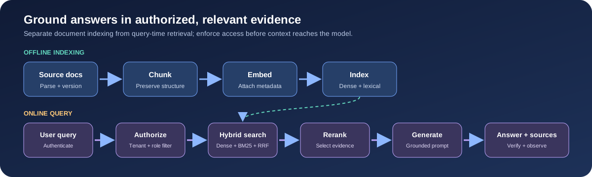
RAG supplies dynamic, verifiable enterprise context at inference time without modifying underlying model weights.

RAG pipeline from source documents through retrieval and grounded response

Advanced RAG Pipeline Enhancements:

Hybrid Retrieval (Dense + BM25): Dense vectors capture semantic intent but miss specific product codes, UUIDs, or part numbers. Production pipelines run dense vector search alongside sparse BM25 lexical search, merging ranked results via Reciprocal Rank Fusion (RRF): $\text{RRF\_Score}(d) = \sum_{m \in \{\text{Dense}, \text{BM25}\}} \frac{1}{k + \text{rank}_m(d)} \quad (k \approx 60)$
Two-Stage Cross-Encoder Reranking: Retrieve a broad candidate set (top 50) via fast ANN vector search, then use an expressive cross-encoder model (e.g., Cohere Rerank, BGE-Reranker) to rescore and narrow down to the top 5 gold passages, eliminating context noise and reducing LLM token costs.

Part III: Production & Advanced AI (Scale & Serving)

3.1 Autonomous LLM Agents & ReAct Orchestration Frameworks

An autonomous agent extends foundation models by interleaving reasoning with external tool execution: $\text{Thought} \longrightarrow \text{Action} \longrightarrow \text{Observation}$

The Four Memory Tiers:

In-Context Scratchpad: Immediate conversational turns and tool returns in the prompt window.
Session State: Distributed key-value cache (e.g., Redis) maintaining active workflow state across turns.
Long-Term Semantic Memory: Vector database storing past interactions and user profiles.
Relational System of Record: ACID SQL databases containing core entity records.

Staff Engineer Rule: Never grant an LLM direct mutate access to high-impact external APIs. Enforce least-privilege tool interfaces, a hard maximum iteration cap (8–10 steps), regex cycle detection, and mandatory Human-in-the-Loop (HITL) gates for financial transactions or data deletion.

3.2 Model Optimization: Quantization, Pruning & Knowledge Distillation

Quantization maps continuous weights into lower-bit representations: $X_{\text{quant}} = \text{clip}\left(\text{round}\left(\frac{X}{S}\right) + Z, q_{\min}, q_{\max}\right)$

FP16 / BF16 (16-bit): 2 bytes/param (Reference baseline).
INT8 (8-bit): 1 byte/param (50% memory reduction with <0.5% perplexity loss).
FP8 (Hopper Native): E4M3 for forward activations, E5M2 for gradients. Supported natively on H100 Tensor Cores, doubling throughput.
INT4 (AWQ / GPTQ): 0.5 bytes/param. Activation-aware Weight Quantization (AWQ) protects salient weights in FP16 while quantizing the remaining 99% to 4 bits, achieving up to 3x memory reduction.

3.3 High-Throughput Serving: vLLM, PagedAttention & Continuous Batching

Autoregressive decoding generates tokens sequentially. Without caching, calculating token $T$ requires recomputing all previous tokens ($\mathcal{O}(T^2)$). Caching past Key and Value tensors reduces per-token decoding to $\mathcal{O}(T)$.

The KV Cache VRAM Formula:

$\text{Memory}_{\text{KV}} = 2 \times 2 \times n_{\text{layers}} \times n_{\text{heads\_kv}} \times d_{\text{head}} \times \text{seq\_len} \times \text{batch\_size} \times \text{bytes\_per\_element}$ For a 70B model (80 layers, 8 KV heads, $d_{\text{head}} = 128$, FP16 = 2 bytes) with 4,096 tokens: $\text{KV\_per\_request} = 4 \times 80 \times 8 \times 128 \times 4096 \times 2 \text{ bytes} \approx 2.68 \text{ GB VRAM per request!}$

PagedAttention & Continuous Batching

Naive KV Cache: Allocates contiguous VRAM based on maximum sequence length, wasting 60%–80% of memory to internal/external fragmentation.
PagedAttention: Manages the KV cache in fixed-size blocks (e.g., 16 tokens) mapped via virtual block tables, mirroring OS virtual memory. Memory utilization exceeds 96%, enabling Prefix Caching across shared system prompts.
Continuous (Iteration-Level) Batching: Admits new incoming requests at each token iteration boundary rather than waiting for an entire batch to finish, yielding a 10x to 24x throughput increase.

3.4 Production Evaluation & Defense-in-Depth Guardrails

Production releases require quantitative gating via the RAGAS Framework:

Faithfulness: $\frac{ \text{Supported Claims} }{ \text{Total Claims in Answer} }$ (Target: $> 0.85$).
Answer Relevancy: Semantic similarity between user prompt and generated response.
Context Precision: Are the most relevant chunks positioned at the top of the context?
Context Recall: Did the retriever fetch all facts needed to produce the reference answer?

Three-Layer Defense Guardrails:

Layer 1 (Input Guardrails): Lightweight classifiers (Llama Guard) and regex scanners blocking prompt injection, jailbreaks, and PII.
Layer 2 (Prompt Boundaries): XML context isolation (<context>...</context>) and role instructions.
Layer 3 (Output Verification): Deterministic JSON schema validators, PII redaction, and hallucination verification.

Part IV: Frontier Scaled Architectures (Elite Self-Study)

14 Frontier Architectural Breakthroughs

Mixture of Experts (MoE) Routing: Replaces dense FFN with parallel expert sub-networks. A gating router directs tokens to the Top-2 experts. Enforces an auxiliary load-balancing loss $\mathcal{L}_{\text{aux}} = \alpha N \sum f_i P_i$ to prevent router collapse.
Multi-Head Latent Attention (MLA): DeepSeek’s breakthrough compressing Key and Value matrices into a compact latent vector $c_t^{KV}$, reducing KV cache memory by over 80%.
Speculative Decoding: A small draft model generates $K$ candidate tokens that the large target model verifies in parallel in a single forward pass, delivering a 2–3x latency speedup without altering output distributions.
Distributed Training (Megatron, ZeRO, FSDP): 3D Parallelism: Tensor Parallelism (splitting matrix rows/cols via NVLink), Pipeline Parallelism (1F1B schedule across nodes), and ZeRO-3 / FSDP (sharding optimizer states, gradients, and weights).
Hardware-Aware FlashAttention: Tiles Query, Key, and Value blocks into high-speed on-chip GPU SRAM, computing online softmax to eliminate memory traffic bottlenecks to High-Bandwidth Memory (HBM).
Post-Training Alignment (RLHF, DPO, GRPO): Progression from PPO (4 models in VRAM: Actor, Critic, Ref, Reward) to DPO (implicit reward without Critic) to GRPO (Group Relative Policy Optimization) which eliminates the Critic network for reasoning models (DeepSeek-R1).
Constrained Structured Decoding: Uses Finite State Machines (FSMs) to mask invalid vocabulary tokens dynamically at each decoding step, guaranteeing 100% valid JSON or SQL schemas.
Long-Context Scaling (RoPE & YaRN): Extends context windows to 128K–1M tokens using NTK-Aware frequency scaling and YaRN interpolation.
Model Merging (SLERP, DARE): Blends multiple specialized fine-tuned models in weight space without retraining using spherical linear interpolation and task-vector arithmetic.
Disaggregated Serving: Decouples compute-heavy prefill workers (processing input prompts) from memory-bandwidth-heavy decode workers (generating tokens).
Test-Time Compute Scaling: Extends inference reasoning using Process Reward Models (PRMs) and search over reasoning traces (OpenAI o1, DeepSeek-R1).
Indirect Injection Defense: Implements dual-LLM architectures (Quarantine parser vs privileged actor) and taint tracking on untrusted strings.
Multimodal Vision-Language: Connects visual encoders (CLIP / ViT) to language decoders using cross-attention projection layers (LLaVA).
Embedding & Reranker Tuning: Fine-tunes bi-encoders using InfoNCE contrastive loss with in-batch hard negative mining and Matryoshka Representation Learning (MRL).

Part V: The AI System Design Playbook & Worked Case Studies

5.1 The 8-Step AI System Design Ladder

Clarify Objective & Metrics: Quantify p95/p99 latency budgets, throughput (QPS), cost constraints, and business KPIs.
Baseline Solution: Define the simplest non-ML / classical ML heuristic that works to establish a baseline.
Data & Retrieval Strategy: Modality, chunking boundaries, hybrid indexing (Dense + BM25), and RBAC filters.
Model Selection & Adaptation: Open-source vs. API, parameter sizing (7B vs 70B), LoRA vs. prompting.
Evaluation Plan: Golden benchmark test sets, RAGAS metrics, and online canary A/B testing.
Serving Infrastructure: vLLM, PagedAttention, Continuous Batching, KV cache VRAM sizing, and quantization.
Failure Modes & Guardrails: Prompt injection, hallucination mitigation, output schema enforcement, and loop caps.
Observability & Continuous Retraining: Data drift tracking (PSI > 0.2), telemetry monitoring, and data flywheel.

5.2 The Staff Engineer Mindset: 5 Questions for Every Architecture

Use these questions to make design decisions explicit instead of listing tools:

What is the measurable objective? Name the user outcome, baseline, and success threshold.
What is the simplest viable alternative? Compare against rules, keyword search, or a smaller model before adding complexity.
Where is the bottleneck? Separate model quality, retrieval quality, network latency, GPU memory, and queueing.
How does it fail safely? Define timeouts, fallbacks, access boundaries, and human escalation for consequential actions.
How will we know it is working? Pair offline evaluation with online outcome metrics, latency, cost, and safety telemetry.

5.3 Senior Interview Red Flags to Avoid

Naming a model or vector database before clarifying the user problem and constraints.
Treating a high benchmark score as proof of production quality without a representative evaluation set.
Assuming retrieved context is trustworthy or that prompt instructions alone enforce tenant isolation.
Optimizing average latency while ignoring p95/p99, queueing, and timeout behavior.
Proposing fine-tuning to inject frequently changing facts that belong in a retrieval system.
Reporting a single aggregate quality metric without segmenting failures by task, language, tenant, or risk.

5.4 Worked Case Study 1: Real-Time Code Completion Engine (<50ms Latency)

Problem: Design an IDE code completion engine for 500,000 DAU with suggestions appearing as developers type.
SLA & Scale: Strict p95 latency < 50ms; peak throughput 15,000 QPS; target developer acceptance rate > 30%.
Baseline: Language Server Protocol (LSP) AST completion (< 5ms) serving as instantaneous fallback.
Context Assembly: Fill-in-the-Middle (FIM) format: <PRE> prefix <SUF> suffix <MID> completion <EOS>. AST symbol extraction fetches recently edited function definitions from active repo tabs.
Model Architecture: Compact 3B parameter model (StarCoder2 3B) quantized to INT8 via AWQ (3.5 GB VRAM footprint).
Serving Architecture: Disaggregated serving with speculative decoding: a 100M parameter draft model speculatively predicts 4 tokens; the 3B model verifies them in parallel in one forward pass (2.4x speedup). PagedAttention caches prompt tokens from common repo header imports.
Guardrails: Secret scrubber stripping API keys; license compliance Bloom filter checking against public GPL code; Tree-sitter AST syntax validator checking bracket closure before rendering suggestions.
Observability: Telemetry tracks accepted vs dismissed completions, logging rejected suggestions for weekly DPO preference alignment retraining.

5.5 Worked Case Study 2: Enterprise Multi-Tenant RAG Copilot with RBAC

Problem: Design a customer support AI assistant for a SaaS platform with 5,000 enterprise tenants, 100M documents, and strict Role-Based Access Control (RBAC).
SLA & Scale: End-to-end response < 1,000ms p95; zero cross-tenant data leakage; RAGAS Faithfulness > 0.95.
Baseline: ElasticSearch BM25 keyword search over tenant ticket databases.
Multi-Tenant Retrieval & RBAC: Logical partitioning in a distributed vector store (Qdrant/Milvus) with metadata payload pre-filtering on the HNSW graph traversal: { tenant_id: 'acme_corp', allowed_roles: { $in: ['tier1_agent'] } }. Vectors from other tenants are mathematically inaccessible during graph traversal.
Retrieval Pipeline: 384-token chunks with 50-token overlap; Parent-Child indexing; Hybrid Search combining dense vector recall with BM25 keyword search via Reciprocal Rank Fusion (RRF); Cross-encoder reranker scoring top-30 candidates down to top-4 gold context passages.
Serving Architecture: Llama 3 70B served via vLLM with PagedAttention and FP8 quantization. Individual enterprise tenants with custom brand voices receive dedicated LoRA adapters (30MB each), dynamically hot-swapped into the serving engine at inference time using Multi-LoRA batching.
Guardrails: Input rail scanning for jailbreaks and indirect prompt injection; XML prompt context boundaries; output rail running automated regex PII redaction and JSON schema validation.
Observability: Weekly audit of RAGAS Context Recall and Faithfulness. Interactions with reranker confidence < 0.4 are flagged for human supervisor review and added to the golden evaluation set.

5.6 Candidate Self-Assessment Scorecard (50-Point Staff Rubric)

| Competency Area | Staff Engineer Benchmark Expectation | Self Score | | :— | :— | :— | | 1. Foundations & Math | Derives scaled dot-product attention variance; explains why stacked linear layers collapse without non-linear activations; distinguishes SGD, Adam, and AdamW weight decay mechanics. | [ ] / 5 | | 2. Transformer Internals | Articulates Query/Key/Value roles; derives RoPE rotational math; explains MHA vs MQA vs GQA memory bandwidth bottlenecks during autoregressive generation. | [ ] / 5 | | 3. Adaptation & LoRA | Calculates VRAM state of AdamW (16 bytes/param); derives LoRA low-rank decomposition (W + BA); explains QLoRA NF4 quantization and multi-tenant adapter hot-swapping. | [ ] / 5 | | 4. Production RAG | Designs end-to-end hybrid retrieval (Dense + BM25 with RRF); implements two-stage cross-encoder reranking; isolates retrieval vs generation failures via RAGAS metrics. | [ ] / 5 | | 5. Serving & Infrastructure | Calculates exact KV cache memory formulas; explains how PagedAttention eliminates internal/external fragmentation; designs continuous iteration batching schedulers. | [ ] / 5 | | 6. Model Optimization | Compares FP16, INT8, FP8 (E4M3/E5M2), and INT4 (AWQ/GPTQ); explains why weight quantization accelerates memory-bound decoding even on modern Tensor Cores. | [ ] / 5 | | 7. Agents & Guardrails | Constructs robust ReAct loops with least-privilege tool schemas, cycle detection, and hard loop limits; designs 3-layer defense-in-depth against indirect prompt injection. | [ ] / 5 | | 8. Frontier Scaled Systems | Explains MoE auxiliary load-balancing loss, DeepSeek MLA latent KV compression, Speculative Decoding rejection sampling, FlashAttention online softmax SRAM tiling, and DPO vs GRPO. | [ ] / 5 | | 9. System Design Structure | Leads the 8-Step System Design Ladder without prompting; asks quantitative SLA questions upfront; articulates the Staff Engineer 5 Questions for every architectural block. | [ ] / 5 | | 10. Production Drift & MLOps | Differentiates data drift from concept drift; computes Population Stability Index (PSI); builds automated telemetry alerts and continuous evaluation CI/CD gates. | [ ] / 5 |

5.7 Must-Read Foundational Papers (The AI Engineer Canon)

Tier 1 (Foundational):
- Attention Is All You Need (Vaswani et al., 2017) — Scaled dot-product attention, multi-head projections, and positional encoding logic.
- BERT (Devlin et al., 2018) & GPT-2 / GPT-3 (Brown et al., 2020) — Bidirectional masked LM vs Autoregressive causal language modeling.
- Retrieval-Augmented Generation (RAG) (Lewis et al., 2020) — Combining parametric generator memory with non-parametric dense vector retrieval.
- vLLM: PagedAttention (Kwon et al., 2023) — Virtual memory paging applied to KV caches, continuous iteration batching, and prefix caching.
Tier 2 (Core Adaptation & Efficiency):
- LoRA: Low-Rank Adaptation of Large Language Models (Hu et al., 2021) — Low-rank decomposition matrices $B \cdot A$ updating <1% of weights.
- FlashAttention 1, 2, 3 (Dao et al., 2022–2024) — IO-aware attention tiling into GPU SRAM with online softmax calculation.
- Direct Preference Optimization (DPO) (Rafailov et al., 2023) — Eliminating Critic and Reward models in RLHF via closed-form loss reparameterization.
Tier 3 (Frontier Scaled Architectures):
- DeepSeek-V3 & DeepSeek-R1 Technical Reports (2024–2025) — Multi-Head Latent Attention (MLA), auxiliary-loss-free MoE routing, and Group Relative Policy Optimization (GRPO) for reasoning.

Part VI: Interview Questions & Answers

Use these as practice prompts: answer aloud first, state assumptions, and then compare your response with the points below. Strong answers connect technical choices to measurable product constraints.

Foundations & Model Selection

1. When would you choose a classical ML model instead of an LLM?

Answer: Start with the task and data. For structured prediction such as churn or fraud scoring, gradient-boosted trees are often cheaper, faster, easier to calibrate, and simpler to audit. Use an LLM when the task genuinely needs language understanding or generation. Compare candidates on a representative holdout set, latency, total serving cost, explainability, and operational burden.

2. What is the difference between data drift and concept drift?

Answer: Data drift is a change in the input distribution, P(X); concept drift is a change in the relationship between inputs and outcomes, P(Y | X). Monitor input statistics continuously, but use delayed labels, outcome metrics, and targeted audits to detect concept drift. A distribution alert is a reason to investigate, not proof that a model should be retrained.

3. Why does a Transformer use scaled dot-product attention?

Answer: Query-key dot products tend to grow in variance with key dimension. Large logits can saturate softmax and weaken gradients. Dividing by the square root of the key dimension controls the scale, helping keep optimization stable. Attention then uses the normalized compatibility scores to mix value vectors.

4. Explain the difference between fine-tuning and in-context learning.

Answer: In-context learning provides examples or instructions in the prompt and changes no model weights; it is quick to iterate but consumes context and may not reliably enforce behavior. Fine-tuning updates model parameters using training examples, which can improve a repeated task or style but requires data quality controls, evaluation, and a deployment lifecycle. Use retrieval for frequently changing factual knowledge rather than trying to memorize it in weights.

RAG & Retrieval

5. A RAG answer is wrong. How do you find the cause?

Answer: Trace the request through the pipeline and inspect the evidence at each stage. Check document freshness and permissions, then measure retrieval recall on a labeled query set. Inspect ranking and reranking, verify the final prompt contains the right passages, and test whether the model follows the evidence. This separates ingestion, retrieval, context construction, and generation failures before changing components.

6. How do you choose a chunking strategy?

Answer: Match boundaries to document structure and the questions users ask. Preserve headings and metadata, and compare fixed-size, sentence-aware, and parent-child approaches on retrieval recall and answer quality. Tune chunk size and overlap empirically: tiny chunks lose context, while large chunks add noise and consume the generation context budget.

7. Why combine BM25 with dense vector search?

Answer: Dense retrieval is good at semantic similarity, while BM25 is often stronger for exact terms such as identifiers, names, and error codes. A hybrid retriever covers both query types; rank fusion such as RRF combines result lists without requiring their raw scores to be directly comparable. Validate the added complexity against a query set that includes both semantic and exact-match cases.

8. What is the purpose of a reranker?

Answer: A fast retriever narrows a large corpus to a candidate set; a cross-encoder then scores each query-document pair jointly to improve ordering. Reranking can improve precision in the final context, but it adds latency and compute. Measure whether that quality gain justifies the cost and keep the candidate set bounded.

Evaluation, Reliability & Safety

9. How would you evaluate a generative AI feature before launch?

Answer: Build a versioned, representative test set that includes common, difficult, and high-risk cases. Measure task-specific correctness, groundedness where relevant, refusal and safety behavior, and latency/cost. Use human review for ambiguous judgments, run regression tests on every prompt/model/retriever change, and launch behind a canary with rollback criteria.

10. How do you mitigate prompt injection in a RAG application?

Answer: Treat retrieved documents and user input as untrusted data. Enforce authorization in the retrieval/data layer, not through prompt wording; give tools narrow, validated permissions; separate instructions from quoted evidence; and require confirmation for sensitive actions. Add adversarial tests and monitor tool calls and policy violations, since no single prompt pattern is a complete defense.

11. What should you do when an AI system’s quality degrades?

Answer: First determine the scope and user impact, then compare recent quality, traffic, data, model, prompt, and index changes against a known baseline. Break metrics down by task and segment, inspect examples, and isolate the failing stage. Roll back or route to a safe fallback when impact is material; retrain only after identifying a data or model issue that training can address.

12. How do you evaluate an LLM-as-a-judge?

Answer: Treat it as a measurement instrument, not ground truth. Write a rubric tied to observable criteria, calibrate judgments against expert-labeled examples, test agreement and known biases, and blind model identity where practical. Keep human review for high-impact cases and track judge drift when the judge or prompt changes.

Serving & System Design

13. What drives LLM inference latency, and how would you reduce it?

Answer: Separate time to first token from inter-token latency. Prompt length and prefill compute affect the first token; model size, memory bandwidth, KV-cache pressure, batching, and queueing affect generation. Profile before optimizing, then consider prompt/context reduction, quantization, efficient batching, caching, or a smaller model while checking quality and tail-latency impact.

14. How would you design a multi-tenant RAG service with strict access control?

Answer: Authenticate the caller and derive tenant and role claims from trusted identity, then apply authorization filters at the data boundary before results reach the model. Partition or scope indexes appropriately, prevent cross-tenant cache leakage, and test adversarial access cases. Log access decisions safely, monitor isolation violations, and make authorization failures explicit rather than silently returning unrestricted results.

15. When should an LLM agent use a tool rather than answer directly?

Answer: Use a tool when the answer depends on current or authoritative external state, or when a bounded action is needed. Keep tool schemas narrow, validate arguments and results, enforce authorization outside the model, and limit retries and steps. For consequential or irreversible actions, require explicit user confirmation and provide a safe fallback.

16. How do you explain a system design trade-off in an interview?

Answer: State the requirements and assumptions, present a simple baseline, and compare alternatives against quality, latency, cost, reliability, and operational complexity. Explain the main bottleneck and failure mode, then define how the design will be measured and rolled back. Be clear about what you would defer until traffic or evidence justifies it.